Siliceous and Delicious

Back at the office. Started the day where I left off yesterday—getting the diversity panel for the disparity/diversity figure together. I had plotted genus and species richness on the same scale, but that really didn’t look great (the genus diversity was basically flatlining), so I think I’ll overplot them on the same frame but at different scales.

I was interrupted by a visit from Tinker, shortly thereafter joined by JC. It was nice to see them (and it had been several days since I talked with either one), but it definitely contributed not insubstantially to the loss of a morning’s productivity (it’s lunch time now, and I’m still only getting started). Clearly, I get more done at a café (ideally one with expensive, non-functioning wireless) than at the office.

That said, the conversation with Tinker and JC was quite helpful—I was talking through my latest plot and Tinker pointed out that, perhaps, my mean-pairwise-distance plot was flatlining because it considers all of the characters, not just the ones with the most variance—which by definition is what should be captured by the first few PCO axes, on which the other measures (convex hull, alpha volume) are based. The test, it occurred to me on thinking this through, would be to plot the mean pairwise distance through time as measured in the space defined by the first 3 PCO axes. If that also shows an increase, then it’s the confounding non-variable characters in the original d-matrix causing the flatness; if the plot however is also flat, then there’s something to be explained.

In any case, I eventually got some reasonably focused time in, though only a fraction of what I achieved yesterday, and finished the four-panel diversity/disparity plot:

It was very gratifying to hear both JC and Tinker ooh and aah over it when they saw it; JC also mentioned that Andy had come by to chat to her and asked, very excitedly, whether she’d seen my plots and how good they looked. And it was loud enough that Tinker heard it, too.

What I would really like to do now—with a view to the insight that struck me at Diesel yesterday—is to set up the code for this figure so that I can generate different versions of it based on different taxon (sub-)sampling algorithms: sampled in-bin, range-through, boundary-crossing (?), naive rarefaction, by-list unweighted subsampling, and of course shareholder quorum subsampling.

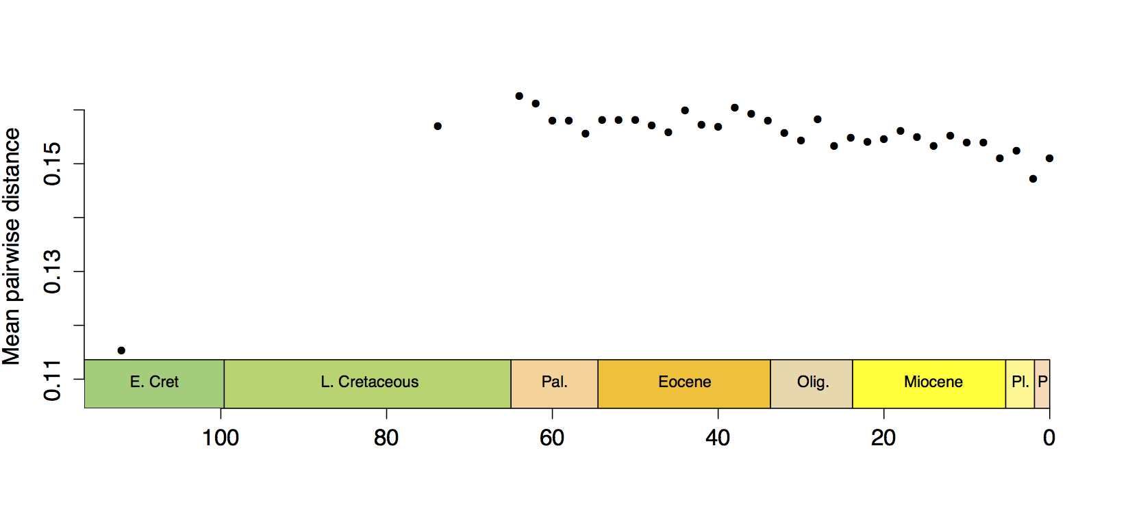
Here, incidentally, is the pairwise distance plot through time using Euclidean distance in PCO space (first three axes only)—showing that disparity is pretty constant through time, by this measure, and it’s not an artifact of using the whole data vs. just part of it.

This is a pretty interesting result I’m going to have to think about (probably best to do that by writing). And need to dig up that Erwin paper… Anyway. Time to go home!