Siliceous and Delicious

Finally—finally!—after far too many days of (admittedly less than full steam) work , R spat out the “specific character sets through time” plot. The idea behind this was to choose a few possible adaptive roles the silica frustule plays in diatoms, and then see if character states deemed more supportive of a particular role became more common through time. For example, supposing the frustule has something to do with defense against predation, we might expect the number of genera with spines, reinforced bars and ribs, more spherical (crushing-resistant) frustules, and so forth relative to those lacking such features to increase through time.

Well, to cut to the chase—for all four functional avenues I explored with my data there is a remarkable absence of any sort of trend through time. They’re all as flat as a dead man’s ECG. Sigh. What a spectacularly poor use of my time! What a disappointment! What a surprise that the very last analysis, for which I was holding onto all of my saved-up hope, the one that was going to give sense and meaning to the whole project, turned out to be a total dud…What a joy to leave this idiotic line of inquiry behind!

Well. Now that I have all this code together (which was trickier to write than I expected), I might as well look at individual characters. Perhaps it’s my choice of characters grouped into the four character sets that is essentially causing a central-limit-theorem-like averaging because they are essentially randomly distributed trends.

Here’s what that plot looks like:

This confirms the suspicion, to an extent. Some characters do have trends, but they’re largely feeble, and by no means consistent. Together that seems to wipe out any trend in taking the average over many characters. Oh well. That’s that!

The end of last week was a bit of a struggle—the accumulated weeks of struggle combined with watching SJ and John Crowley defend (in the same day) drove the point of my stasis home with a vengeance. It was a bit of a low.

It was doubly pleasant and important, then, that the weekend was a real raiser of spirits. On Saturday Kati and I got away for the day, spent a very relaxing morning talking at Darwin’s, and then a restorative afternoon walking through Maudslay State Park in Newburyport. It gave us the chance to finally spend the sort of quality, pair-bonding, unstructured and carefree time together that I had hoped Copenhagen would provide, but was disappointed that it hadn’t. Perhaps it just needed time, but things feel markedly improved this morning.

On Sunday afternoon we spent some time with Evan and Katie (and Gavi), which was also a surprising source of motivation. Evan has an almost uncannily positive attitude to big tasks and intimidating projects at work. Perhaps it was because I came primed from a weekend of relaxing and connecting, but somehow giving my usual “no, I’m not done yet” pity party spiel this time inspired me to take a more Evan-ish, optimistic, go-gettum view of the task at hand. I am at a point where I can finish up (these first two chapters, at the very least), and what a formidable challenge. So, instead of moping, fearing, and pushing my head far into the sand until the last moment of the weekend, I actually spent Sunday evening quietly looking forward to getting to work and moving forward. I programmed the coffee maker before bed and felt rested and ready to go this morning.

Anyway, this is all a long preamble, but the bottom line is that I am working at Darwin’s today feeling qualitatively different than I have for the past few months—since the big push started petering out in March.

I left off yesterday with a cliffhanger about the conceptual jump from a simple 1D space of character states to the “number of realized pairwise character combinations” disparity metric. This metric takes the 1D list of character states and expands it to two dimensions, with two identical axes. Each grid square (matrix element) is now a combination of two characters, the matrix representing all possible pairwise combinations. Some of these pairwise combinations need to be disregarded, of course. For starters, the main diagonal of the matrix represents pairings of a character state with itself, which obviously makes no sense. So from a total of (m^2) combinations, we must subtract m items. Then, because the matrix is symmetric, we must disregard one half of the remaining combinations, because the upper triangle is a duplication of the lower triangle, leaving [(m^2)-m]/2 combinations. Finally, some of these remaining combinations will be impossible—for examples, pairwise combinations of states of the same character (you can’t be square and triangular at the same time, using yesterday’s example), as well as logically inapplicable combinations (from my morphospace, for example, you can’t have “no raphe” and “fibulae” at the same time). So the final number of combinations can be written as something like  {[(m^2)-m]/2} – k. Crucially, this number is of order (n*x)^2 rather than the “full” morphospace, which for binary characters has 2^n, for multistate characters x^n where n is the number of characters and x is the number states for each, and so on.

So, to cut a long story short—there are three ways I’ve talked about to measure how much morphospace is occupied. The first is to measure how many “cells” of the full, n-dimensional morphospace are occupied, but this is such a vast space that changes in occupancy are likely to be meaningless. And more importantly, a nightmare to try and calculate. The other extreme is to simply collapse the morphospace down into 1 dimension, namely a binary space consisting of just the character states. This will be much less sparsely filled. Somewhere in between those two options, but closer to the second one, is the “realized pairwise character combinations” approach. It will be more sparsely occupied than the 1D approach, but much more densely occupied than the full morphospace. But: it’s no different in principle than the 1D approach, and I think it only really makes sense if the 1D approach fails because the data “saturate” in 1D (like in our toy example).

Here’s the justification why I’m not going to go through the trouble of doing pairwise states: The number of realized states tops out at about 300 (306 to be exact). My plot shows an increase through time up to that point. There are 317 states in total, so we are not “saturating” that 1D space early—I think we’re seeing everything we’re going to be able to see. Justification, part II: it would be a ton of work and a genuine hassle to figure out which are the forbidden character combinations (due to logical inapplicability). [BUT: this might not actually be necessary, since that’s only required to tally the total number of possible pairwise combinations, e.g. for calculating % saturation of the space. Wouldn’t be needed for a tally of the raw number of realized pairwise combinations.]

It’s been a slow trickle coming back from Denmark. I have been writing a bit more in my document (see the results here), but then decided that a better way to go was to write topic sentences for paragraphs/main points out onto index cards to be subsequently arranged into a logical order, the first attempts at which I have also been sketching out (in an actual notebook, with an actual pencil).

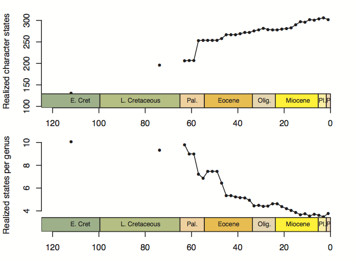
This afternoon I finally bit the bullet, booted up R, and started the final couple of analyses and plots. I think I’d been holding onto them as a last resort of “I know what I’m doing” type of tasks before the truly gaping maw of writeup uncertainty. That last resort is now dwindling. Here is the plot for the number of realized character states, including a panel standardized by the number of genera in each time bin:

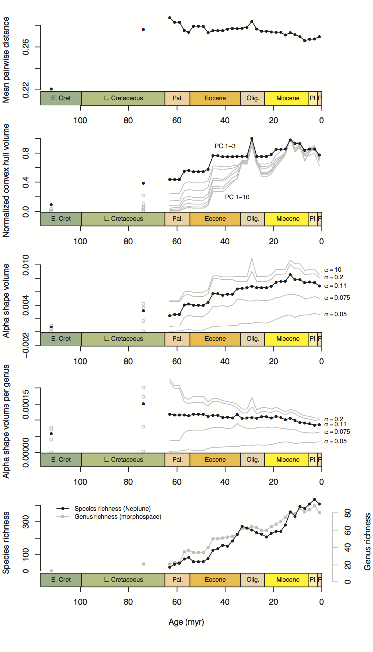
The number of realized states goes up, unsurprisingly. This agrees with the PCO volume metrics (convex hull/alpha shape volume). When divided by the number of genera, though, the realized states go down—meaning each genus contributes less “raw” morphospace individually as time goes on. This I think reflects the same thing as the mean pairwise distance plot, which also goes down through time (at least a bit)—more and more taxa are being packed into the occupied volume of morphospace, and it’s happening more quickly than the expansion of morphospace itself.

One of the remaining plots I had on my list to do was the “number of realized pairwise character combinations” through time, mostly because I had read it used in a few different places (including the review by Ciampiglio, the review by Erwin, and at least one of the Foote papers), but I had not understood what it meant. I spent some time yesterday reading about it, and I think I get it now. But I am not sure if I want to bother to do it.

Here’s my best stab at explaining what the “realized pairwise character combinations” are. First, it helps to think about what a morphospace of discrete characters looks like, or at least can be thought of. Let’s start in lower dimensions. In 2D, we can think of a morphospace with just two characters, say color (red, green, or blue) and outline (square, circle, or triangle). This could look like a 2D grid, or matrix, where each square can be occupied or unoccupied by an organism.

-          Red   Green   Blue

Square      X              X

Circle             X

Triangle                   X

In this example, we have red and blue squares, but no green squares, blue triangles but no red circles, and so on. Now we have two characters with three states each, and six character states in total. But there are nine possible pairwise character combinations. Let’s add another character. If we add limbs to this—with states one or two—we get an additional dimension, or two “layers” of these nine combinations for a total of eighteen possible configurations of organisms. The more dimensions (characters) we add, the more sparsely occupied the morphospace will be for any given number of organisms. For example, in our 2D space we could realize all possible morphologies with 9 organisms, if they were all different; for the 3D space we would need 18. Add another character with four states, say, and now we need 72… so as you can see for a large space such as mine, the number of possible combinations becomes huge.

In my case, I’m not sure what it is exactly, but assuming an average of 3 states per character and 123 characters, that’s 3^123, or 5 x 10^58. That’s somewhere between the estimated number of stars (10^23) and the number of atoms (10^80) in the universe. So, with about 140 taxa, a very sparsely populated space. So comparing how the space in its full dimensionality fills up through time doesn’t make much sense—it’s going to go from being basically empty to being basically empty.

So what to do?

What I’ve done in the graphs above is to collapse that hyperdimensional space into just one dimension—think of it as a linear row of boxes, each box representing a character state, either filled or unfilled. How many boxes are filled through time? For the toy example above, it would look something like this:

Red   Green  Blue  Square  Circle  Triangle  One limb  Two limbs

X       X      X     X       X        X         X

Clearly, this is an easier space to fill! In the toy example, I’ve assumed there are no two-limbed things, only one-limbed things… In any case, that’s the idea for the plots I posted above. Now, here comes the conceptual jump for the pairwise character combinations!

Made this plot, following on from the plots showing average list length through time and average convex hull volume per list through time. It struck me that they looked similar, and indeed, when time is taken out of the equation and one is plotted against the other, it seems indeed that the major control on morphospace occupied by a list is the diversity of that list (at least when viewed on average per time bin).

What does this mean? Well, in the most conservative (and perhaps cynical) interpretation, I would read this to mean that morphospace is pretty well constant over time. Some lists are longer than others, perhaps because of the choice of what taxa to list for a particular section, or perhaps because there were simply fewer taxa present in the section. But the more taxa are found, the more morphospace is occupied. The two outliers are, of course, the Cretaceous samples (data collected according to very different rules), the rest fall on a pretty tight trendline.

Progress report season… for the sixth time! Yay! Well, actually I’m not sure I even had a progress report the first two years, but whatever. I spent yesterday evening reading through the past year’s DSA notes (depressing), comparing them to the goals I set out at this time last year (actually, precisely to the day!). This morning, I sat down and wrote out the progress report and handed it to Andy. I was feeling pretty good about myself, particularly since I managed to convince him not to call a committee meeting (for the first time ever). But then he read over the report and came back to my office to request a change: I had described how, as per his recommendation, I was dropping the diatom diversity project and instead expanding the morphospace project to two chapters, he “reminded” me of the PlanktonTech book chapter we agreed to write and asked that I change the section in my progress report back to include a chapter on diatom diversity.

What?! I thought the diatom diversity chapter was dead. I thought I had explained to Andy that I didn’t think the SQ subsampling method was going to work on the Neptune data. I thought he had suggested I drop the chapter, “with an eye toward finishing sooner rather than later”. Well, that didn’t seem to matter much—I suppose he remembered that there was a book chapter due for the PlanktonTech people, and that it was supposed to be about diatom diversity, and that was it. Just add it to the dissertation, as another chapter.

I could freak out at this point. I could despair about how to goalposts keep shifting. I could sit down and try to realistically plan how I am going to go from two chapters worth of data and analysis and no chapters written to four chapters worth of data and analysis and four chapters written by September 15th (the deadline for dissertation submission for the November graduation date). But I think I’m just too exhausted to do that at this point. Andy wants a chapter on diversity? Fine. So I rewrite the progress report (here it is, by the way) to include a few sentences about how “the diatom diversity project will take on a smaller role and will be represented by a short review chapter for submission to the book resulting from the PlanktonTech research initiative”.

Whatever. I don’t have the energy to engage with stressing out about how long things are going to take, when I am going to be done, what the dissertation is going to look like. The best I can do right now is go from one day to the next. Today, I needed to get a progress report done and signed by my committee members. I did that—I got Andy, Jacques, and Dave to sign off on it (and without requiring a committee meeting!). Whatever happens tomorrow, or next month, or when the thesis is due, happens then. Who cares what the damn report says.

I have been trying, but every step just seems to be met with a branch in the face. I have been working on code since yesterday to calculate the morphospace volume occupied by individual lists, a sort of “alpha disparity”, but it keeps crashing on me (as in, just quitting R). I can’t figure out what’s wrong. It just makes me seethe. The code is the least, the tiniest of my problems. Yet it alone, at this point of almost complete demoralization, seems capable of defeating me.

Spent HOURS trying to debug this fucking code. Was able to eventually narrow it down to a call to the function that calculates convex hull volume, presumably because it is passing short lists to the function (i.e. it is failing when trying to compute the 3D hull volume of a point set of only 3 points). This is a real arse of course because if I have to reject lists with 4 or fewer taxa in them I’m clearly going to overestimate morphospace occupancy. Fuckity fuckity fuck. God, I hate this shit.

Anyway, that hack seemed to make it work, but the results are neither expected nor really clear.

So, actually it looks like this measure of “disparity” at one location is going DOWN with time, if anything. That is not what I would have expected, neither from the overall morphospace pattern, nor from what’s out there about diatoms in the abstract. Things should have evolved to a greater diversity of forms, even in one location, not less.

So does the list length (number of species at a location) go down with time, to explain this? No. Of course not. That would be too fucking easy.

 So it looks like, if anything, list length goes up. Although, really, list length is basically constant. This makes nothing clearer to me, nothing at all.

Finally forcing myself, on an overcast Sunday, to pick up the pieces, and grudgingly drag myself forwards. Item one: alpha volume per genus. This shows demonstrates my reasoning from before, that mean pairwise distance decreases through time because there’s more taxa crammed into a growing space, but the taxon-cramming exceeds the rate of space growth.

The largest alpha value is of course the same as the convex hull, and here we see the best correspondence with mean pairwise distance. Instead of mean pairwise distance, though, this is mean volume of morphospace occupied by each taxon. Which is about the same thing. The next question arising, then, is what does the mean volume occupied by a list, i.e. an ODP site, look like through time? This would be one way of looking past sampling issues and at least look at the disparity in one location through time.

Took the day off to see Tufte do his thing. It was cool. I liked the idea of making graphics about the content, and putting everything in service of the cognitive task at hand—of making every aspect of the display support the intellectual activity the display is trying to accomplish. At many points along the way I reflected on what this means my morphospace project. In some ways, a helpful reflection. In other ways, reinforcing my crippling stuckness. There’s nothing I can accomplish with a good figure if I don’t know what I’m trying to say with that figure.

The metaphor is the map. Make the graphic as clear and uncluttered and minimal as a map. But, how can you make a map if you don’t know where you’re going?

“The best good design can do is not to get in the way.” I liked that thought. But it scared me a bit, too, because in some ways I feel like well-designed figures is all I have in this project. What I’m lacking is the spine to back it up.

The sun is out, it’s forecast to be in the 70s today and up to 80 tomorrow. It’s the first day of spring. I’m sitting outside Darwin’s in a t-shrt, it feels wonderfully fresh and warm, and yet there’s something holding me back from really enjoying it. What, oh what could that be…

I feel totally paralyzed, still, by that question Zoe asked on Friday. What can you say about your results? I just don’t know. What are the two points do I want to make? What am I trying to say? What question is this morphospace project answering? Fuck.

Beau helped tremendously in DSA today. Somehow, talking it all through crystallized for me that there’s only one way out, and that’s through me. The help is going to come from nowhere, so I need to muscle my own way through it. Asking for help, being humble and self-critical and loyal to the truth is going to get me nowhere. I’ve had the best results in the past when I’ve been confident, self-assured, argued by advocacy and basically played the part of the blowhard. That’s just what I’ll have to do to get through this.