Siliceous and Delicious

In spite of my heroic efforts—dragging myself to work on labor day, an achievement that required forsaking a morsel of  socialist integrity—my attempts at setting up another overnight run of the FIB were thwarted by a “suppressor below limit” warning, which made obtaining any sort FIB image an impossibility. Thereby rendering the whole exercise impossible from the get-go. The upside was that I regained my labor day, the downside that I have nothing new to report from the FIB.

This morning I bit the bullet and finally replied to Dave’s email, meanwhile a week old, apologizing profusely for any offense I may have caused in my request of the full Neptune database, and proffering up my effusive thanks for the file he did provide. I’ll discuss the situation with Andy in our next meeting (perhaps Friday?) and see what he says, besides of course trying to decipher whatever runes constitute Dave’s reply.

I decided to return to Friday’s question of the three-timer statistic, which turned out so differently than I had expected. Did I do something wrong with it? I thought I might compare my curve to what’s in the Rabosky paper, but in his supplements, the only thing he shows is the sampling probability for each of the subsampling exercises (rather than the overall sampling probability, as I have calculated, for the raw data).

If I didn’t do anything wrong, then the huge differences between the curves in my three-timer graph and the SIB/RT graph must lie in one- and two-timers, which I think is the only difference between the two counts. However, this difference would inflate the total diversity considered in SIB/RT and make the relative difference (between SIB and RT, analogous to the difference between 3T and 3T+PT) smaller… so, at the end of the day, the SIB/RT ratio should be higher than the 3T/(3T+PT) ratio. Which it isn’t! It’s lower, and a lot more variable. That variability I don’t think I can attribute to one- and two-timers, because any addition of those entities to the SIB count will also show up in the RT count, and vice versa.

Perhaps the way to tackle the question of whether the algorithm is actually doing what it’s supposed to do, I’m best off doing what I did with the SIB/RT algorithm: make sure the 3T and PT are being calculated properly by adding lines to the function to return those values along with the final %age. Did this, and couldn’t find much of anything out of the ordinary that would suggest something was going horridly wrong. The only low %ages are in time bins 47 and 48 (32% and 3%, respectively), everything else is above 70%. Unlike in the SIB/RT calculation. Here’s another view of the graph (same as last post’s), but with the x-axis expanded:

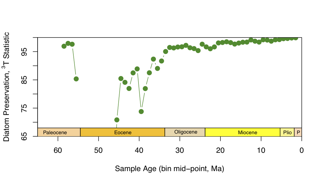
Don’t know what to do beyond this. It is what it is, report to Andy, move on? One final thing I could do, I suppose, is correct for the edge effects by comparing the focal bin to the adjacent time bins only, rather than comparing to everything before and everything after. Here’s the outcome (not much different, as is plainly clear):

Again, “preservation” (or “sampling probability”, as I think Alroy calls it) is pretty steady at between 95-100%, with some dips in the Eocene, and a little one in the early Miocene (which doesn’t show up in the long-range three-timer plot above, presumably because the missing taxa in the bins adjacent to the ~22 Ma time bin with the low %age are present elsewhere in the data set, from whence they can be ranged through).

The siren howled a little earlier this afternoon, in recognition of Beaudry’s imminent departure. It’ll be a tough start to the working day tomorrow knowing my DSA buddy is an ocean away. For today, I’m calling it quits.

Started the day on an upswing after the last week of downward spiraling. Took a trip to the VWR store to pick up the tools needed to fashion my own little desiccator—some Drierite and a couple of little screw-top plastic tubs—and made some more samples for this afternoon’s rescheduled pre-FIB SEM session. The Drierite didn’t end up doing much, but I found that placing the stubs directly under a lamp helped things tremendously. Ah, the simple pleasures in life.

That done, I found myself with nothing left to do on the FIB front (the day’s scheduled project) until the afternoon. I decided to get cracking on the now months-old ‘1-pager-for-Charles’ task. Finally replotted the diversity plot I had marred with my mistyping of the Cenozoic stage boundaries, but didn’t get much else done, mired in the bugs of my R code. Crap. Stopped for lunch to read the lab meeting paper for tomorrow.

In the afternoon, checked those FIB samples. A few of them (the finer grained fraction) looked like hell, don’t know how I’m going to prep those samples to make it work. The coarser ones were OK and I was able to rank them in order of promisingness for tomorrow’s overnight session (19C looked best, then 27C, then 25C).

As my office is now allegedly under reconstruction*, I convened bright and early (well, at least reasonably early) at Darwin’s to start the week in a hopefully productive fashion. Had to faff around for about half an hour to find a decent description of the day’s first target, Cladogramma. Am feeling a little nervous about just how long this is taking me. I think I might need to step it up a gear and really put in hours here—a familiar theme from months and now even years past. Not sure how to make that actually happen amidst all the other things going on and my general disinclination for hard work.

Spent another half an hour, this time without any sort of success at all, searching for any sort of information at all about the next species, Clavicula. Started getting incredibly, unbelievably frustrated. Where am I supposed to be looking? Surely there must be descriptions of these genera out there somewhere for all of those diatom taxonomists to use? Where the fuck are they? Who the fuck am I supposed to ask? I am alone on a fucking island, and I fucking hate it. Went with the crappy-assed 19th-Century description in the Van Heurck text and moved on. Who cares? Nobody is going to give a shit about this anyway, and I just need to get myself out of this nightmare.

Bolli had a short paragraph about Cosmiodiscus, which according to AlgaeBase contains only one valid species (C. insignis). Pictures added from a DSDP initial report furnished enough of a description to keep things moving.

Quit this after lunch to prepare some more samples for this afternoon’s pre-FIB SEM session. This turned out to be an epic fail, because the samples didn’t dry before I was due to sputter coat them before the SEM session on the Zeiss EVO. I had simply assumed that the vacuum of the sputter coater would draw off the moisture—but this turned out to be an idiotic assumption, as the only thing the water did was begin violently boiling and frothing, without actually evaporating. I had to rush back to the office and cancel the SEM session and put this all off for another day. Fuckity crapshit.

*Note that no construction worker actually showed up during the entire day. The office is unoccupied, empty, and not being worked on at the moment.

The morning somehow, magically, disappeared into a long run and a proof-read of Ben Gill’s Toarcian OAE paper. Once I got myself into work, had lunch, and worked my way through the administrative chores (emails, setting up a FIB overnighter for next week, etc), I was into a good part of the afternoon.

The plan for today called for diatom FIB, but as I’m de-emphasizing this project after my last conversation with Andy, and am waiting for the first overnight session next week (as well as waiting for the diatom culture to be harvested by the CCMP), I thought I’d return to the sample selection exercise I’d been making such good progress on yesterday.

Was interrupted by the arrival of our new postdoc, Erik, who asked for some help bringing his filing cabinet up to the office. An offhand remark of his threw me off and served a bit of a major motivational blow for the rest of the afternoon.

Morning flew by—had to read a paper and try to find a book in the ed school library (without success) for the new “Old Thymes” journal club. What had started out as a nice discussion a couple of weeks ago amongst five senior graduate students today seemed to have crossed the attendance threshold of meetings beyond which all usefulness seems to transform directly into completely unproductive dickwaving. In the parlance of our times.

I slipped out through the door and made my way to the FIB, for a session on how to do the automation business. It seems to be fairly straightforward, much like doing the milling manually, except you set up a list of milling operations beforehand and mark their location with “x”-shaped registration marks. It’ll take a couple of hours (more like three) to set up in the evening (maybe 3-6 pm?), and then I’ll need at least an hour (probably more like two) for debriefing (and taking images) afterwards in the morning (Maybe 7-9 am?). We’ll see how it turns out, I’m certainly not getting my hopes up.

This all left me with no time for the actual supposed task for the day, which was to work on the morphospace.

Spent the morning talking to a fresh-faced undergraduate visiting the department as a prospective graduate student. After that, a rather late start. It being time for the fossil diatom FIB project, I’m largely still stuck here. I am waiting to meet Nicholas on Monday about automation, and I need to find a way to select more samples for analysis, too.

Made another sample in preparation for Monday, in the hope that it would have a better density of complete frustules, and decided to throw in the towel again, being that I was feeling like crap, didn’t know what to do next, and had no motivation to think about what that might be.

Started the day with a characteristically cathartic and constructive DSA meeting, followed by a lengthy lunchtime hiatus in honor of Tais’ last day at work. In the afternoon I met with Andy, going a long way towards resolving some of the issues and anxieties discussed with Beau in the morning. Some concrete outcomes of the meeting:

1. As regards the morphospace, Andy thinks my approach of linking morphometric data to Neptune is “spectacular” (his words), and thus worth the effort, even if this means putting in a fair amount of work tracking down obscure descriptions of fossil genera.
2. After hearing my complaints about the difficulties of the FIB work, Andy stated that he believed the morphospace, diversity/e-o, and radiolarian projects would make “three valuable chapters”, which I understood to mean ‘sufficient for a thesis’, and that I may decide at the end of the summer that the FIB project would be something I’d save for a post-doc.
3. Andy was very engaged by my re-telling of Alroy’s SQ algorithm and continues to think that the E-O project will make an “interesting and important” thesis chapter.

Knowing that the FIB project is not a requirement for graduation immediately transformed my perception. Suddenly—without the pressure of feeling that I have to do it—the FIB project seems infinitely less depressing and daunting, and much more like a challenging adventure. It’s funny how the mind works. All in all, a great day of meetings… and that’s not something you hear often!

Spent the morning on the FIB with the engineer in charge, Nicholas Antoniou. He was very helpful and trained me in how to stigmate, focus, and align apertures on the various ion probes in the FIB. It’s a monumentally finicky process, but I think I get the basic picture of what needs to be done now. However, once we’d gone through this exercise, it became clear in a) a couple of trial milling operations we carried out using the now perfectly-tuned ion beams, and b) the conversation we had throughout, that using the higher-current beams (which would reduce the milling time from many—as many as dozens of—hours per specimen to a slightly more reasonable hour or so) is simply not an option. No matter how well adjusted the beams, the 23 and 45 nA probes produce an ion beam that is simply not sharp enough to cut open the frustule cleanly—the result is an unevenly cut frustule caked in ‘curtaining’, step-shaped deposits, and other milling artifacts.

This, needless to say, was a heavy blow. The probe sizes which gave halfway decent results (delivering 6.5 and 13 nA of current) will take countless hours (on the order of a day or two) to cut through the larger frustules I’m currently working with (the Cretaceous sample I’m looking at at the moment, for example, has frustules in the 100 µm length range). It’s simply beyond the size range of what the FIB is designed to efficiently handle (it’s really set up to work with nm- to few-µm size features on electronic chip circuits).

There was some moderately good news, though it was hard for me to really get excited about it. Nicholas talked at the end about the possibility of setting up automated milling operations overnight. This approach would involve milling registration marks (“X marks the spot”!) next to frustules to be milled, which are then sequentially found using pattern recognition in the course of a night’s automated milling. The FIB locates the desired feature on the stub and aligns it using the registration marks, then carries out a pre-set milling operation, then moves on to the next registration mark, and so on. Theoretically this would make very long milling operations (at least on the order of several hours) more feasible.

The amount of time this implies, though, is still staggering. Assuming I can mill 2 or 3 specimens overnight, this will still require on the order of 100 nights of milling to generate measurements for the 50% taxonomic coverage case I suggested in my thesis proposal. This is patently ridiculous, in spite of being a probably wildly over-optimistic assessment of how much time it’s actually going to take to make these measurements.

I’m distraught and demotivated. Nothing seems to want to work at the moment. For better or worse, we have an early lab meeting this afternoon—a dull paper about some early Proterozoic pyrite concretions that are suggested to be biological, maybe even multicellular and (heresy!) eukaryotic in origin. In any case, daft and dreary as it may be, I’m going to have to spend the remainder of the day reading the assigned papers, so I don’t look like any more of a fool in front of my advisor. Yech.